How to use Imaris to check if the Spots Accumulate around the Surface

Imaris has a new analytical tool within Vantage, called Spatial View Plot. Using it you can try to answer the question if your Spots objects accumulate around the Surface of another object, which might later be interpreted as an interaction or explained by other biological phenomenon. In Imaris we try to answer this question by comparing the observed distribution of Spots with the random (simulated) distribution of Spots. 

First thing first, to do this analysis you need to detect one of your objects, here microglia as Spots and other object, here vasculature as a Surface. Please remember to check the box Object-object statistics in the first step of every creation wizard. I will quickly run the detection using the stored values. For your object detection, adjust the segmentation parameters to your sample. 

As you see, just by looking at the dataset there’s no obvious answer my question: do microglia spots accumulate around blood vessel surface,  

So I open the Spatial View Plot in Vantage to show you what numbers Imaris has calculated in the background. 

The starting point of this analysis is the measurement and representation of the Histogram count plot, which shows the calculated number of Spots within the distance d from the Surface. There are 3 options of the histogram, which show the values: Inside, outside and both in and outside of Surface. In my case – I’ll select outside of surface option.  

The X axis of the plot shows the Shortest distance to Surface and Y axis – the number of spots at any given distance d. So here I can read there’s around 11 Spots found at 10 micrometers distance from the Surface. In Imaris you can as well find this plot counterpart – Cumulative count plot where we see the cumulative number of spots within a distance d from the surface.

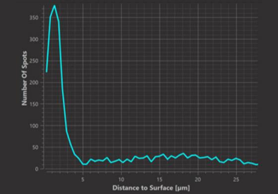
Histogram Plot (at distance d)

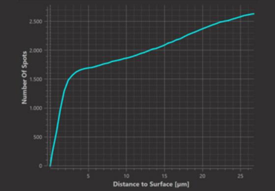
Cumulative Plot (within distance d)

In the background, Imaris 9.7 randomly throws the same number of Spots into the same 3D volume and adds the results to both Histogram count plot and Cumulative count plot. The results of this simulations are added to the plot when you click the option “Show complete spatial random generated data” and represented as a dashed line surrounded by a shaded region. It’s important to understand that there were 1000 simulations made.  98% of those simulations gave the result within the shaded region while 1% of the simulations gave the result above the shaded region and 1% below.  

Since the simulated spots are by construction randomly distributed and neither accumulate nor are repelled from the surface, they provide a useful null hypothesis and deviations from this null hypothesis indicate attraction or repulsion.

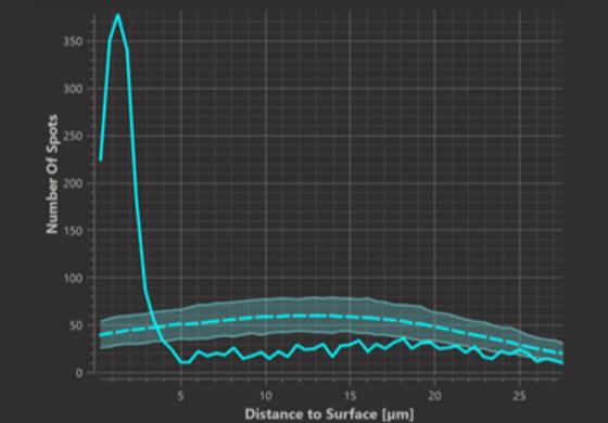
Histogram Plot (at distance d)

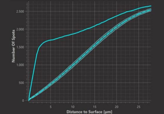
Cumulative Plot (within distance d)

Within the Cumulative count plot, where the observed cumulative function is above the simulations it indicates that the observed number of spots within the respective distance to the surface is greater than what is expected from random simulations, so we can call it  “accumulation or attraction”. Where the observed cumulative function is lower than the simulations it indicates that the observed number of spots within the respective distance to the surface is lower than what is expected from random simulations, which we can explain as repulsion from the Surface.  

In the histogram count plot on the other hand we can observe at which distances from the surface spots occur in greater or lesser numbers than expected from random distribution. In this example I see that the Histogram function is very rough which in this case is caused but small number of data points, but we can already observe some trend of accumulation up to around 20 micrometers from the Surface.  

To help statistical inference in the situations where number of observed (and simulated Spots) is to small to produce a smooth plot (visible ups and downs), we have added the Probability density plot and Cumulative density plot (CDF), which represent the density of Spots at or within a given distance respectively. Those plots give similar information as their original counterparts: Histogram and Cumulative count plot but are statistically smoothed using a kernel density estimate. Both observed and randomized plots are smoothed in the same manner. The kernel width is displayed in the legend of the graph.   

To answer the question within which distance around the Surface Spots are accumulated, we will here use the smoothed Probability Density plot. It’s now good to remind that from 1000 simulations, 98% of the simulated Spots were enclosed within the randomization envelope  - the shaded region.  Thus it’s plausible to reject the null hypothesis that our observed Spots  are distributed randomly,  when the observed curve lies outside of the randomization envelope.  

Imaris also proposes a calculated parameter called attraction distance which is positioned where the observed curve crosses the randomized curve. Based on this distance you can conclude that the observed Spots are accumulated within the attraction distance from the Surface.